Example 1a: GridLAB-D as a Value Federate
HELICS messages that are value-oriented are the most common type of messages. As mentioned in the federate introduction, value messages are intended to be used to represent the physics of a system, linking federates at their mutual boundaries and allowing a larger and more complex system to be represented than would be the case if only one simulator was used.
Value Federate Interface Types
There are four interface types for value federates that allow the interactions between the federates (a large part of co-simulation/federation configuration) to be flexibly defined. The difference between the four types revolve around whether the interface is for sending or receiving HELICS messages and whether the sender/receiver is defined by the federate (technically, the core associated with the federate):
Publications - Sending interface where the federate core does not specify the intended recipient of the HELICS message
Named Inputs - Receiving interface where the federate core does not specify the source federate of the HELICS message
Directed Outputs - Sending interface where the federate core specifies the recipient of HELICS message
Subscriptions - Receiving interface where the federate core specifies the sender of HELICS message
In all cases the configuration of the federate core declares the existence of the interface to use for communicating with other federates. The difference between “publication”/”named inputs” and “directed outputs”/”subscriptions” is where that federate core itself knows the specific names of the interfaces on the receiving/sending federate core.
The message type used for a given federation configuration is often an expression of the preference of the user setting up the federation. There are a few important differences that may guide which interfaces to use:
Which interfaces does the simulator support? - Though it is the preference of the HELICS development team that all integrated simulators support all four types, that may not be the case. Limitations of the simulator may limit your options as a user of that simulator.
Is portability of the federate and its configuration important? - Because “publications” and “named inputs” don’t require the federate to know who it is sending HELICS messages to and receiving HELICS messages from as part of the federate configuration, it affords a slightly higher degree of portability between different federations. The mapping of HELICS messages still needs to be done to configure a federation, its just done separately from the federate configuration file via a broker or core configuration file. The difference in location of this mapping may offer some configuration efficiencies in some circumstances.
Though all four message types are supported, the remainder of this guide will focus on publications and subscriptions as they are conceptually easily understood and can be comprehensively configured through the individual federate configuration files.
Federate Configuration Options via JSON
For any simulator that you didn’t write for yourself, the most common way of configuring that simulator for use in a HELICS co-simulation will be through the use of an external JSON configuration file. TOML files are also supported but we will concentrate on JSON for this discussion. This file is read when a federate is being created and initialized and it will provide all the necessary information to incorporate that federate into the co-simulation.
As the fundamental role of the co-simulation platform is to manage the synchronization and data exchange between the federates, you may or may not be surprised to learn that there are generic configuration options available to all HELICS federates that deal precisely with these. In this section, we’ll focus on the options related to data exchange as pertaining to value federates, those options and in Timing section we’ll look at the timing parameters.
Let’s look at a generic JSON configuration file as an example with the more common parameters shown; the default values are shown in “[ ]”. (Further parameters and explanations can be found in the federate configuration guide.
Example 1a - Basic transmission and distribution powerflow
To demonstrate how a to build a co-simulation, an example of a simple integrated transmission system and distribution system powerflow can be built; all the necessary files are found HERE but to use them you’ll need to get some specific software installed; here are the instructions:
Python - Anaconda installation, if you don’t already have Python installed. You may need to also install the following Python packages (
conda install…)matplotlib
time
logging
PyPower -
pip install pypower
This example has a very simple message topology (with only one message being sent by either federate at each time step) and uses only a single broker. Diagrams of the message and broker topology can be found below:


Transmission system - The transmission system model used is the IEEE-118 bus model. To a single bus in this model the GridLAB-D distribution system is attached. All other load buses in the model use a static load shape scaled proportionately so the peak of the load shape matches meet the model-defined load value. The generators are re-dispatched every fifteen minutes by running an optimal power flow (the so-called “ACOPF” which places constraints on the voltage at the nodes in the system) and every five minutes a powerflow is run the update the state of the system. To allow for the relatively modest size of the single distribution system attached to the transmission system, the distribution system load is amplified by a factor of fifteen before being applied to the transmission system.
Distribution system - A GridLAB-D model of the IEEE-123 node distribution system has been used. The model includes voltage regulators along the primary side of the system and includes secondary (or distribution) transformers with loads attached to the secondary of these transformers. The loads themselves are ZIP loads with a high impedance traction that are randomly scaled versions of the same time-varying load-shapes.
In this particular case, the Python script executing the transmission model also creates the broker; this is a choice of convenience and could have been created by any other federates. This simulation is run for 24 hours.
Running co-simulations via helics run ...
To run this simulation, the HELICS team has also developed a standardized means of launching co-simulations. Discussion of how to configure a JSON for use in launching a HELICS-based co-simulation is discussed in the over here but for all these examples, the configuration has already been done. In this case, that configuration is in the examples folder as “cosim_runner_1a.json” and looks like this:
{
  "broker": true,
  "federates": [
    {
      "directory": ".",
      "exec": "python 1abc_Transmission_simulator.py -c 1a",
      "host": "localhost",
      "name": "1a_Transmission"
    },
    {
      "directory": ".",
      "exec": "gridlabd 1a_IEEE_123_feeder.glm",
      "host": "localhost",
      "name": "1a_GridLABD"
    }
  ],
  "name": "1a-T-D-Cosimulation-HELICSRunner"
}
Briefly, it’s easy to guess what a few of these parameters do:
“directory” is the location of the model to be run
“exec” is the command line call (with all necessary options) to launch the co-simulation
With a properly written configuration file, launching the co-simulation becomes very straightforward:
helics run --path=<path to HELICS runner JSON configuration file>
Experiment and Results
To show the difference between running these two simulators in a stand-alone analysis and as a co-simulation, modify the federate JSON configurations and use helics run ... in both cases to run the analysis. To run the two as a co-simulation, leave publication and subscription entries in the federate JSON configuration. To run them as stand-alone federates with no interaction, delete the publications and subscriptions from both JSON configuration files. By removing the information transfer between the two they become disconnected but are still able to be executed as if they were participating in the federation.
The figure below shows the total load on the transmission node to which the distribution system model is attached and the transmission system voltage at the same node over the course of the simulated day.
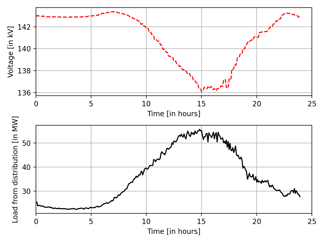
As can be seen, the load and voltage are correlated as expected but the correlation is relatively weak; big changes in load have minimal impacts on the transmission voltage. This is what we would expect for a simple transmission and distribution co-simulation.